Author: Axel Almet
introduction, installation, and data download
Here, we will integrate four datasets of human pancreas cells from different studies. This collection has been used to benchmark a number of integration methods now and is used in the following Scanpy tutorial.
It’s also worth mentioning that a lot of what I will run here is per the guidelines of the benchmarking comparison by Luecken et al. (2020). The code that was used to obtain the results in Luecken et al. can be found at the following GitHub repository.
First thing’s first, let’s install Scanpy, Scanorama, and, if you’d like to compare Scanorama’s performance with a similar method, BBKNN.
!pip install scanpy
!pip install scanorama
!pip install bbknn
# The following packages should already be part of Google Colba
import numpy as np
import pandas as pd
import matplotlib.pyplot as plt
import scanpy as sc
import scanorama as scrama
Obtain the Pancreas dataset used in the Scanpy tutorial.
# If you want to see how many cells there are:
pancreas_all = sc.read('data/pancreas.h5ad', backup_url='https://www.dropbox.com/s/qj1jlm9w10wmt0u/pancreas.h5ad?dl=1')
pancreas_all
AnnData object with n_obs × n_vars = 14693 × 2448
    obs: 'celltype', 'sample', 'n_genes', 'batch', 'n_counts', 'louvain'
    var: 'n_cells-0', 'n_cells-1', 'n_cells-2', 'n_cells-3'
    uns: 'celltype_colors', 'louvain', 'neighbors', 'pca', 'sample_colors'
    obsm: 'X_pca', 'X_umap'
    varm: 'PCs'
    obsp: 'distances', 'connectivities'
To be honest, I don’t know what to do about the NaNs in the genes below. If anyone has a good idea for this, I’d love to hear it.
pancreas_all.var # To demonstrate that not every batch recorded the same genes.
| n_cells-0 | n_cells-1 | n_cells-2 | n_cells-3 | |
|---|---|---|---|---|
| index | ||||
| A2M | 273.0 | 120.0 | 262.0 | 635.0 |
| ABAT | 841.0 | 988.0 | 1052.0 | 635.0 |
| ABCA1 | 418.0 | 623.0 | 468.0 | 635.0 |
| ABCA17P | 63.0 | NaN | 104.0 | 635.0 |
| ABCA7 | 410.0 | 74.0 | 1096.0 | 635.0 |
| ... | ... | ... | ... | ... |
| MIR663A | NaN | NaN | 492.0 | NaN |
| LOC100379224 | NaN | 65.0 | 125.0 | 635.0 |
| LOC100130093 | NaN | 228.0 | 764.0 | 635.0 |
| LOC101928303 | NaN | NaN | 533.0 | NaN |
| COPG | NaN | NaN | NaN | 635.0 |
2448 rows × 4 columns
data processing
According to Luecken et al., Scanorama (and in general, other integration methods) are improved by subsetting the data on the set of highly variable genes. We use the CellRanger “flavour” provided in Scanpy. Let’s take the top 1000 highly variable genes. The Scanpy team in general recommends anywhere between 1000 and 5000 HVGs, so you can play with this.
target_genes = 1000
sc.pp.highly_variable_genes(pancreas_all, flavor='cell_ranger', n_top_genes=target_genes, batch_key='batch')
/usr/local/lib/python3.6/dist-packages/statsmodels/tools/_testing.py:19: FutureWarning: pandas.util.testing is deprecated. Use the functions in the public API at pandas.testing instead.
  import pandas.util.testing as tm
/usr/local/lib/python3.6/dist-packages/scanpy/preprocessing/_highly_variable_genes.py:504: FutureWarning: Slicing a positional slice with .loc is not supported, and will raise TypeError in a future version.  Use .loc with labels or .iloc with positions instead.
  df.loc[:n_top_genes, 'highly_variable'] = True
We check the number of HVGs that are highly variable across all $N$ batches. If we do not have enough, we will iterate, taking HVGs from the next \(N-1\), $N - 2, \dots$ batches, until we have the desired number, as specified by target_genes.
# As we don't have enough target genes, we need to consider the 'next best' HVGs
n_batches = len(pancreas_all.obs['batch'].cat.categories)
# These are the genes that are variable across all batches
nbatch1_dispersions = pancreas_all.var['dispersions_norm'][pancreas_all.var.highly_variable_nbatches > n_batches - 1]
nbatch1_dispersions.sort_values(ascending=False, inplace=True)
print(len(nbatch1_dispersions))
176
# Fill up the genes now, using this method from the Theis lab
enough = False
hvg = nbatch1_dispersions.index[:]
not_n_batches = 1

# We'll go down one by one, until we're selecting HVGs from just a single batch.
while not enough:

    target_genes_diff = target_genes - len(hvg) # Get the number of genes we still need to fill up

    tmp_dispersions = pancreas_all.var['dispersions_norm'][pancreas_all.var.highly_variable_nbatches == (n_batches - not_n_batches)]

    # If we haven't hit the target gene numbers, add this to the list and we repeat this iteration
    if len(tmp_dispersions) < target_genes_diff:

        hvg = hvg.append(tmp_dispersions.index)
        not_n_batches += 1

    else:

        tmp_dispersions.sort_values(ascending=False, inplace=True)
        hvg = hvg.append(tmp_dispersions.index[:target_genes_diff])
        enough = True
We can now subset the data on the highly variable genes.
pancreas_all = pancreas_all[:, hvg] # Filter out genes that do not vary much across cells
This step does not actually need to be done, as you can see in pancreas_all.obsm that the PCA and UMAP have already been calculated. But I’ll show it for completneess
sc.tl.pca(pancreas_all, svd_solver='arpack') # Calculate the PCA embeddings
sc.pp.neighbors(pancreas_all) # Determine the kNN graph
sc.tl.umap(pancreas_all) # Calculate the UMAP
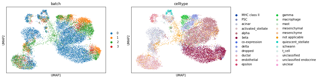
sc.pl.umap(pancreas_all, color=['batch', 'celltype']) # We plot the cell types as well, since it's been already processed.
Trying to set attribute `.uns` of view, copying.
Scanorama requires us to split the data by the batch/sample, so we will do so now.
pancreas_split  = []

for batch in pancreas_all.obs['batch'].unique():
    pancreas_split.append(pancreas_all[pancreas_all.obs['batch']==batch].copy())
In general, one can choose to scale the data, as Luecken et al. do. I’ve found for my own work that it doesn’t make a difference on integration.
running Scanorama
We’re now ready to run Scanorama. Scanorama has two main functions, correct and integrate, and their Scanpy equivalents, correct_scanpy and integrate_scanpy, respectively. The former method is intended for batch correction, while the latter is intended for data integration. There is a distinction between the terms, as described in this paper, but there is probably more overlap than the terms suggest. However, there are a couple of differences between these methods, as described here.
For both methods, a lower-dimensional embedding is calculated, called obms['X_scanorama'], which is to be used instead of PCA. For batch correction, the gene expression matrices are also transformed and returned. If one wants to perform both batch correction AND integration, one sets the option return_dimred=True.
Another difference is that when running integrate, one can also obtain a ‘representative subset’ of the data using geometric sketching. For those on the mathematics sides of things, the differences between sampling via geometric sketching vs sampling on the data itself is kind of like the difference between the Riemann and Lebesgue integral, respectively. The idea is that geometric sketching produces a better representation and accounts for rarer cell types. One can then use this sketch as a reference for futher integration/analysis. This is also particularly useful if the full dataset is quite large and one wants to speed up computation. For more details on geometric sketching, please see the following paper by Hie et al. (2020)—it’s one of the only papers in a Cell journal that I’ve seen contain a proof!
# Now we run Scanorama on the split data.
corrected = scrama.correct_scanpy(pancreas_split, return_dimred=True)

# Merge the corrected datasets
pancreas_all_corrected = corrected[0].concatenate(corrected[1:])
pancreas_all_corrected.obs_names_make_unique(join='_')
To remind ourselves, let’s look at how well integrated the data are before Scanorama.
# Before scanorama
sc.tl.pca(pancreas_all, svd_solver='arpack')
sc.pp.neighbors(pancreas_all)
sc.tl.umap(pancreas_all)
sc.pl.umap(pancreas_all, color=['batch', 'celltype'])
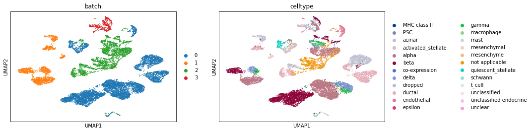
We now use Scanorama’s embedding instead of PCA.
# Now rerun this with Scanoramaa
sc.pp.neighbors(pancreas_all_corrected, use_rep='X_scanorama')
sc.tl.umap(pancreas_all_corrected)
sc.pl.umap(pancreas_all_corrected, color=['batch', 'celltype'])
... storing 'celltype' as categorical
... storing 'sample' as categorical
... storing 'louvain' as categorical
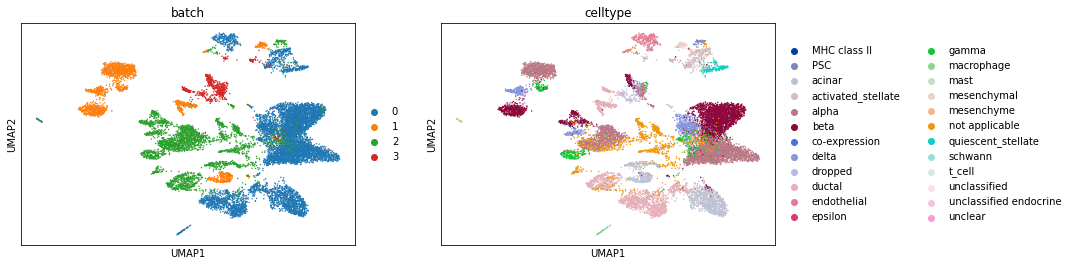
Ta-da! The batches are better integrated with Scanorama. For comparison, let’s also run BBKNN on this (I actually suspect BBKNN will do better).
sc.external.pp.bbknn(pancreas_all, batch_key='batch') # This replaces sc.pp.neighbours and is run on PCA.
sc.tl.umap(pancreas_all)
sc.pl.umap(pancreas_all, color=['batch', 'celltype'])